Answer
As demonstrated in the attached packaged workbook, please find the steps below:
1.Change Mark type to Pie.
2. Configure the sheet to fit the Entire View.
3. Add Sub-Category to Color.
4. Add SUM(Sales) to Angle.
5. Right-click SUM(Sales) in Angle and select Quick Table Calculation > Percent of Total.
6. Right-click Sub-Category in Color and select Sort. Configure it as follows:

7. Drag SUM(Sales) in Angle and drop it to the Data pane. Name it Percent of Total.
8. Create a calculated field and name it Top 4 Label for Sub-Category:
IF RANK_UNIQUE([Percent of Total]) <= 4 THEN ATTR([Sub-Category]) END
9. Create a calculated field and name it Top 4 Label for Percent of Total:
IF RANK_UNIQUE([Percent of Total]) <= 4 THEN [Percent of Total] END
10. Right-click Top 4 Label for Percent of Total and select Default Properties > Number Format. Change the number format to Percentage.
11. Add Top 4 Label for Sub-Category and Top 4 Label for Percent of Total to Label.
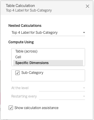
12. Right-click Top 4 Label for Sub-Category in Label and select Edit Table Calculation. Configure it as follows:

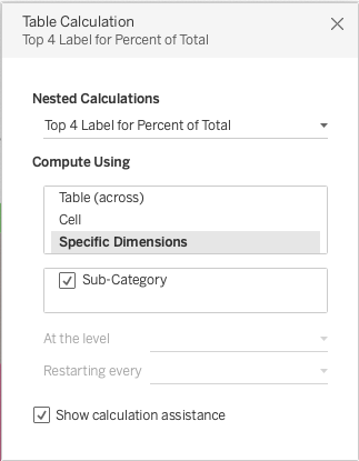
13. Right-click Top 4 Label for Percent of Total in Label and select Edit Table Calculation. Configure it as follows:
